back
Skin growth in the computer
Cells multiplied on the computer screen (in the computer memory), and the transformation of the form was observed. Function alignment was given to an individual cell, and the transformed location of other cells that were pushed by the cells after division was calculated. Cell- multiply method is like an algorithm that seems to move a lot of pinball balls. The division condition was controlled with various kinds of parameters. The method of two dimensions was made first, and the extension to three dimensions was added.
Outline of programming code
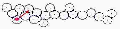 Fig. s1
1- Distance between all cells is measured from a division cell
2- New cell keeps 1 dot apart from a division cell
3- Nearest cell overlapping each other is extracted
4- Direction after pushing is calculated
5- Location of cell is corrected not to be overlapped
6- This process is done on all the cells
Setting of parameter
Main parameters
X coordinate of individual cell
Y coordinate of individual cell
Radius of individual cell
Division determination of individual cell
Division direction of individual cell
The history which is divided of individual continuation
All program codes for skin growing (beta) for MS Basic compiler
Extension to three dimensions
Addition of Z coordinate
A calculation by three dimensions of shift direction
View making with affin transformation
It is transformation to macroscopic image as brightness cline with altitude on z side
 Fig. s2
Course of growth
Size of cells is fixed
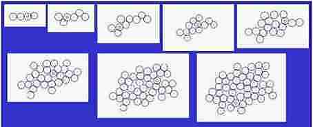 Fig. s3
Size of cells is changeable
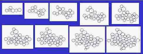 Fig. s4
Course of growth like epidermis
The parameters on the horny layer and in the basal layer are added
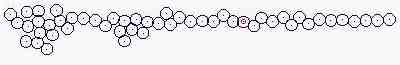
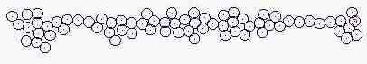

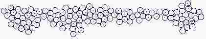
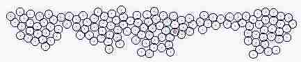
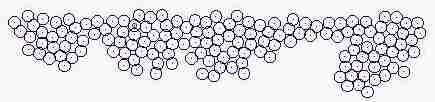
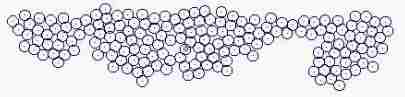
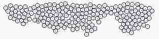 Fig. s5
Setting of parameters in the codes of "Course of growth like epidermis"
r = 5 'radius * *
tate = 50 ' height * *
yoko = 200 ' width * *
allcell = 30 'cell number * *
basee = 14 * *
squat = 30 ' distanse to corneal layer * *
buNRET = 0 ' frequency of division 0 to 1 * *
PRP = 3 'difference of cell size in division. 3 means changeable width of -1.5 to +1.5 * *
kakkak = 360 'Division angle 180= 0 to 180 * *
kakkakA = 360 ' Division angle after division 180= 0 to 180 * *
' XZX = 9 ' 0 - 9 ü© 0 - 180 // 0 - 18 ü© 0-360 * *
ddj = 10 'Division frequency with the same range * *
LAT = .1 'frequency of prohibition to divide after successive division * *
kakNN = .7 ' elasticity of horny layer 0 to 1 , 1 = max. * *
corn = .3 'elimination frequency of horny layer - at squat level : 0 to 1 , max 1 * *
cornda = .2 'elimination frequency of horny layer - not relation to squat level :0 to 1 max=1 * *
mazx = 1 üenumber of horny layer of tornning off * *
gzg = .9 ' frequency of division in only basal layer : 0 to 1 :max= 1 * *
Mass dimension
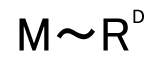
M : area
R : radius
D : Mass dimension
 Fig. s6
Mass dimension is a kind of fractal dimension that presents
the tendency of enlargement of the area.
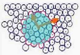 Fig. s7
In the cell growth simulation author used the another method applied of mass dimension.
M (area) is set as the summation of the area of the cells that overlap the circle with R.
Then M '(area) is defined as the inside area of the pink circumference as Fig. s7 in this study.
| Table s1 |
| Log (M ' ) | 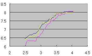 |
| Log ( R ) |
An inclination of the line on Table s1 is D ' (dimension applied of Mass dimension ).
(The values on Table s1 are relative value, not the absolute value)
Measurement of D ' (dimension applied of Mass dimension ) in the cell growth
simulation with fixed and changed cell size
| Fig. s8
| 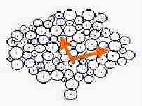 Fig. s9 Fig. s9 |
| |
The definite difference was not found in dimension (D ') between fixed and changed cell size.
Coefficient of variation of Log (M ')/Log (R)
Coefficient of
variation of
Log (M ')/Log (R) | 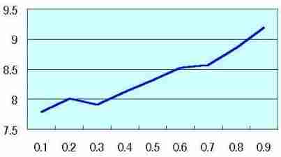 Table s2 Table s2 |
| Probability of the cell size change at one division of cell (0 to 0.9) |
Log (M ')/Log (R) was measured by each R as Fig. s7 and Table s1, then temporary D ' were made by each R.
Coefficient of variation of Log (M ')/Log (R) = ST /(DF / n)
DF = TD1 + TD2 + .... TDn
TDm = temporary D ' by each R
n = total number of measured temporary D '
ST = standard deviation of TDm
Coefficient of variation of Log (M ')/Log (R) was measured by each probability. Coefficient of variation was low in probability 0 ( as Fig. s8 which may mean no mitosis ), and coefficient of variation increased along the rise of probability ( as Fig. s9 which may show the high mitotic status).
(The values on the vertical axis of Table s2 are relative value, not the absolute value)
Simple fractal dimension of the circumference
Simple fractal
dimension of
the circumference |  Table s3 Table s3 |
| Probability of the cell size change at one division of cell (0 to 0.9) |
In the cell growth simulation (as Fig. s7) simple fractal dimension of the circumference ( shown as the pink circumference of Fig. s7) was measured by each probability of the cell size change at one division of cell (0 to 0.9). The vertical axis of Table s3 is the average of simple fractal dimension calculated by each R.
Analysis of histological sturucture of pigmented nevus (clonal type)
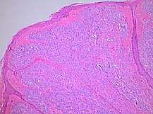 Fig. s10 Fig. s10 | 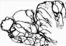 Fig. s11 Fig. s11 |
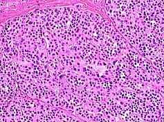 Fig. s12 Fig. s12 | 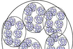 Fig. s13 Fig. s13 |
The possibility of the mathematical representation of naves structure was examined.
Fig. s12 is the magnified figure of Fig. s10, and Fig. s11 is the figure of the walls surrounding each level of cluster of Fig. s10. Fig. s13 is a suppositional figure modeling the cluster of clonal naves. Mathematically formula 1 is led. The structure of Fig. s10 can be made by the cell division of seven times of nine to eleven cells in the first cluster.
RR = rr n x (1 + 1 / cos(90-180/m)) --- formula 1
RR : Radius of the outermost cluster
rr : Radius of the initial cluster
n : Grade number of cluster
m : Number of cells constructing the initial cluster
| RR | 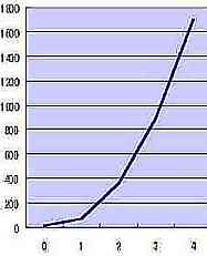 Table s4 Table s4 |
| n |
Log(RR)
+ RR 1/2x 0.1 | 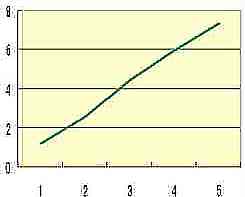 Table s5 Table s5 |
| n |
Table s4 presents the exponential increase of RR that is the average RR of Fig. s11 corresponded to n. The additional formula ( RR 1/2x 0.1 ) on the vertical axis of Table s5 satisfies formula 1 (mathematical simulation), and RR 1/2x 0.1 may show the elasticity or rigidity of the tissue of the skin.
back